Lecture 2: DC Motor Characteristics
Permanent Magnet DC Motors
It makes more sense to discuss advantages and disadvantages of these motor types when we have covered other DC and AC motor types, but broadly speaking permanent magnet DC motors are small in size, relatively cheap to produce and are typically efficient.
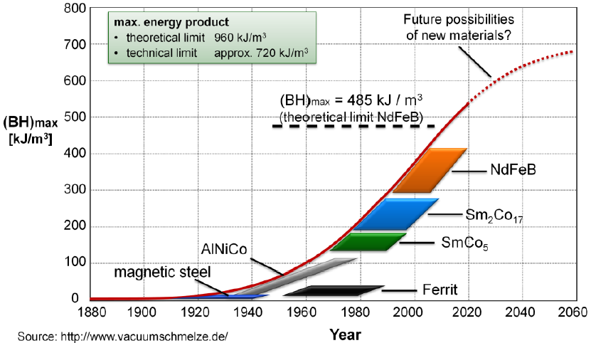
However, permanent magnets are typically limited on the flux density they can produce relative to electromagnets.
Notwithstanding these limitations, there are a number of alternative configurations of permanent magnet DC motors, all based on the fundamental principle described here. These include coreless designs, a variety of winding configurations, ‘pancake’ flat designs etc.
Aside
Research into permanent magnets has increased in recent years, due in part to the advent of electric cars.
Characteristic Motor Data
The characteristic motor data describe the intrinsic motor design and are independent of the applied voltage or current. They reflect the mechanical dimensions, the strength of the permanent magnet and the type of winding used.
Typical values can be found in the specification sheet for a given motor.
- Strongly winding dependent values (electromechanical)
- armature/terminal resistance \(R_a\)
- terminal inductance \(L\) — usually ignored
- torque constant \(K_m\)
- speed constant \(K_b\)
- Almost independent of winding (mechanical)
- speed-torque gradient \(\Delta n/\Delta T_m\) or \(\Delta\omega/\Delta T_m\)
- mechanical time constant \(\tau_m\)
- rotor mass inertia \(J\)
Note: notation may vary depending on the supplier.
Winding Resistance
| Low Resistance | High Resistance |
|---|---|
| thick wire, few turns | thin wire, many turns |
| low rated voltage | high rated voltage |
| high rated and starting currents | low rated and starting currents |
| high specific speed \((\text{min}^{-1}/\text{V})\) | low specific speed \((\text{min}^{-1}/\text{V})\) |
| low specific torque \((\text{mNm}/\text{A})\) | high specific torque \((\text{mNm}/\text{A})\) |
Torque Constant
Produced torque is proportional to motor current:
\[ T_m = K_m\, i_a \]
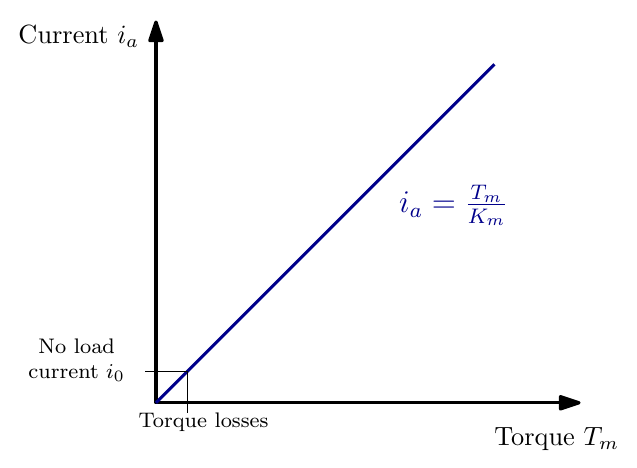
- Defined by motor geometry and magnetic flux densities.
- Torques can be measured by measuring the current.
- For the motor: torque \(\equiv\) current.
- Unit: \(\text{mNm}/\text{A}\) or \(\text{Nm}/\text{A}\).
Back e.m.f and Speed Constant
\[ \varepsilon_b = K_b\,\omega \]
\[ n = K_s\,\varepsilon_b \quad \text{or} \quad n_0 = K_s\,V \]
- Induced back e.m.f \(\varepsilon_b\) is proportional to motor speed \(\omega\).
- law of induction: changing flux in a conductor loop
- induced voltage proportional to speed
- Back e.m.f constant \(K_b\)
- Can be used to calculate rotational velocity for a known back emf
- Is equivalent to \(K_m\)
- Speed constant \(K_s\)
- mostly used for calculating no-load speeds \(n_0\)
- unit: \(\text{min}^{-1}/\text{V}\), i.e. rpm / V
Note: \(n\) is measured in rpm as most data sheets deal in rpm. From an engineering perspective angular velocity is measured in rad/s and is denoted \(\omega\). Care should be taken to use appropriate units.
Back e.m.f. and Armature Current
The supply voltage is shared between the back e.m.f. and the voltage drop across the winding resistance:
\[ V = \varepsilon_b + i_a R_a \quad \Rightarrow \quad i_a = \frac{V - \varepsilon_b}{R_a} \]
- At switch-on the rotor is still, so \(\varepsilon_b = 0\) and only \(R_a\) limits the current: the large stall (starting) current \(V/R_a\).
- As the motor speeds up, \(\varepsilon_b\) rises and the current falls: they move in opposite directions along a straight line of slope \(-1/R_a\).
- At no-load speed \(\varepsilon_b\) is almost equal to \(V\) and only the small no-load current flows. Adding load slows the motor, lowers \(\varepsilon_b\) and lets more current flow to make the extra torque.
Interactive version: Back e.m.f. and current · Open full screen ↗
Speed Torque Curve
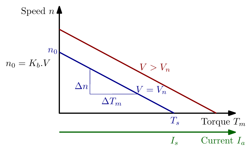
| Symbol | Meaning | Symbol | Meaning |
|---|---|---|---|
| \(V\) | applied voltage (V) | \(I_s\) | stall current (A) |
| \(V_n\) | nominal voltage (V) | \(T_m\) | motor torque (mNm) |
| \(n_0\) | no load speed (rpm) | \(K_b\) | speed const. (\(\text{min}^{-1}/\text{V}\)) |
| \(T_s\) | stall torque (mNm) | \(n\) | motor speed (rpm) |
Increasing the applied voltage shifts the speed–torque line upwards, parallel to itself: the gradient \(\Delta n/\Delta T_m\) is a property of the motor and does not change with voltage.
Speed Torque Gradient
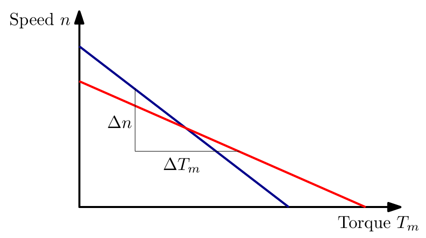
| Weak Motor (blue) | Strong Motor (red) |
|---|---|
| steep speed-torque line, high \(\Delta n/\Delta T_m\) | flat speed-torque line, low \(\Delta n/\Delta T_m\) |
| sensitive to load changes | not sensitive to load changes |
| e.g. weak magnet, smaller motor | e.g. strong magnet, larger motor |
Winding Type
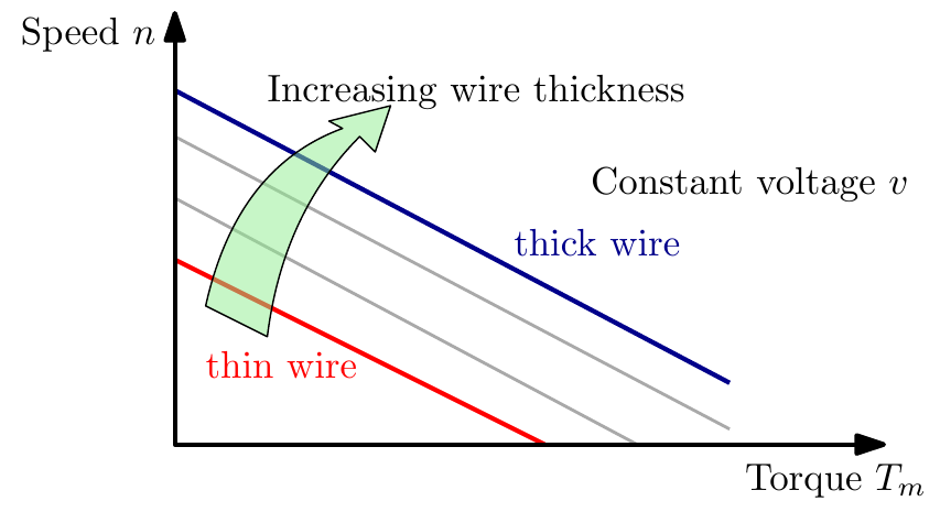
There are numerous winding types; varying the winding at the design stage can adjust for:
- electrical input power (voltage, current of power supply)
- mechanical output power (speed, torque)
For a permanent magnet DC motor the speed torque curve is effectively a constant for a given winding series.
Speed, Torque, Power and Efficiency
Typical values for motor constants/properties can be found in the specification sheet for the motor. Let’s take a look at the specification sheet of the motor below and plot some key curves and motor efficiency.
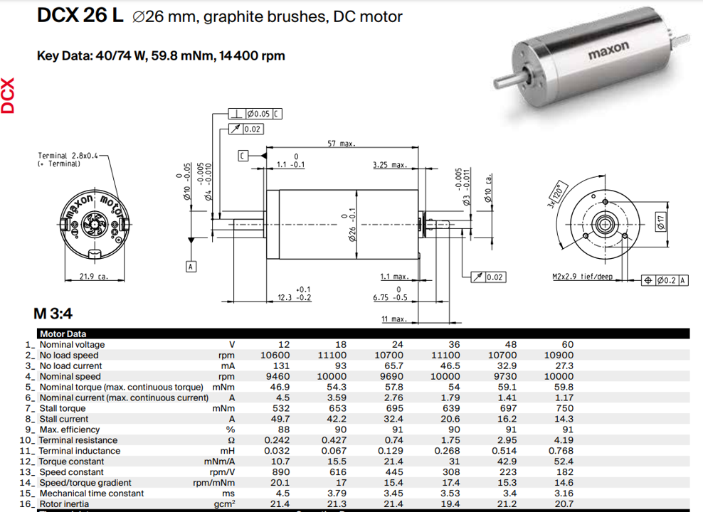
DC Motor Power
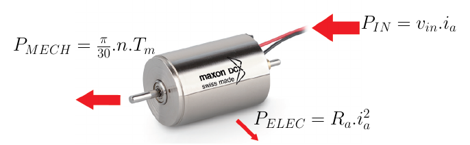
\[ P_{IN} = P_{MECH} + P_{ELEC} \]
\[ P_{MECH} = P_{IN} - P_{ELEC} \]
\[ P_{OUT} = P_{IN} - P_{Losses} \]
Where:
\[ P_{IN} = v_{in}\, i_a, \qquad P_{MECH} = \frac{\pi}{30}\, n\, T_m, \qquad P_{ELEC} = R_a\, i_a^2 \]
There are a number of different ways to calculate efficiency; among the simplest, assuming the motor is running at a steady angular velocity, is:
\[ \eta = \frac{P_{MECH}}{P_{IN}} = \frac{\frac{\pi}{30}\, n\, T_m}{v_{in}\, i_a} = \frac{v_{in}\, i_a - R_a\, i_a^2}{v_{in}\, i_a} \]
Where \(n\) is the speed in rpm and all other terms are as described in the previous sections.
The factor \(\pi/30\) converts speed in rpm to angular velocity in rad/s: \(\omega = \dfrac{2\pi n}{60} = \dfrac{\pi}{30}\,n\).
Case Study: Maxon DCX 26 L
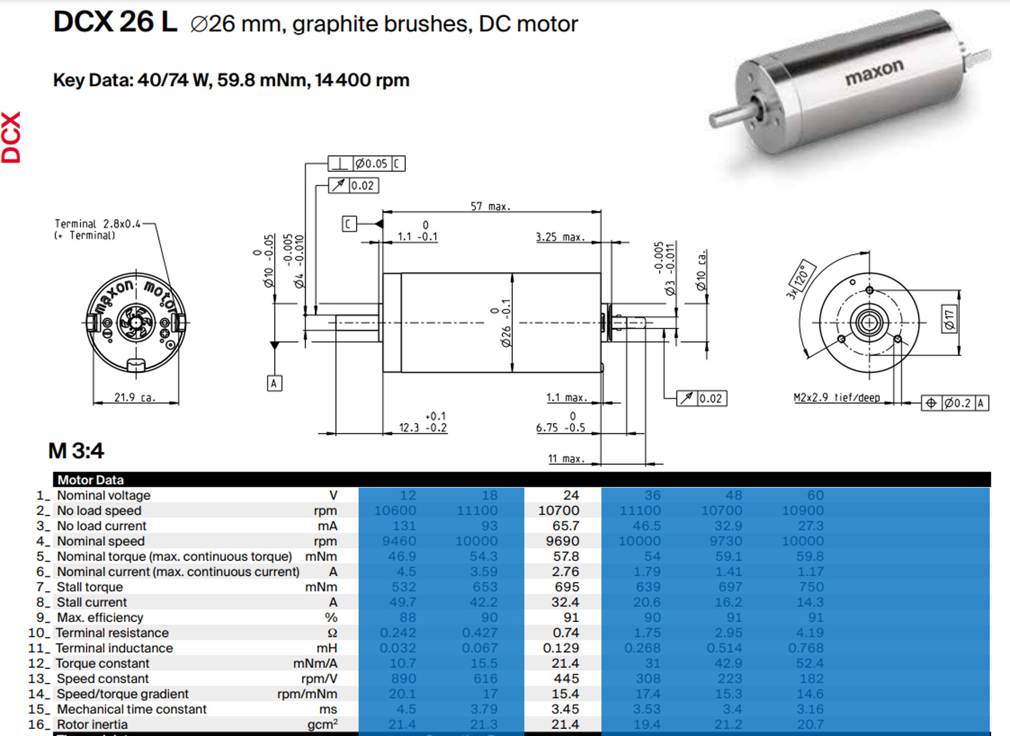
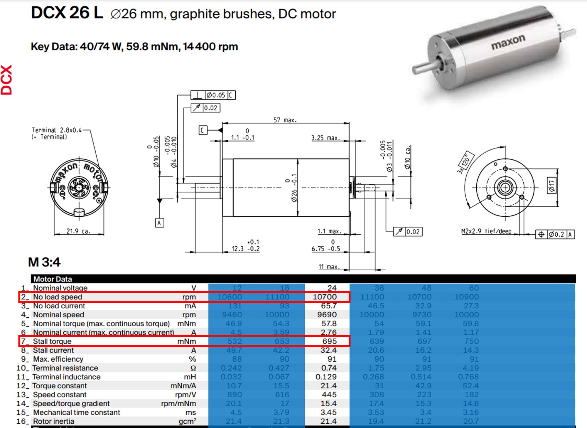
DCX 26 L — Ø26 mm, graphite brushes, DC motor. Key data: 40/74 W, 59.8 mNm, 14 400 rpm.
Speed and power against torque
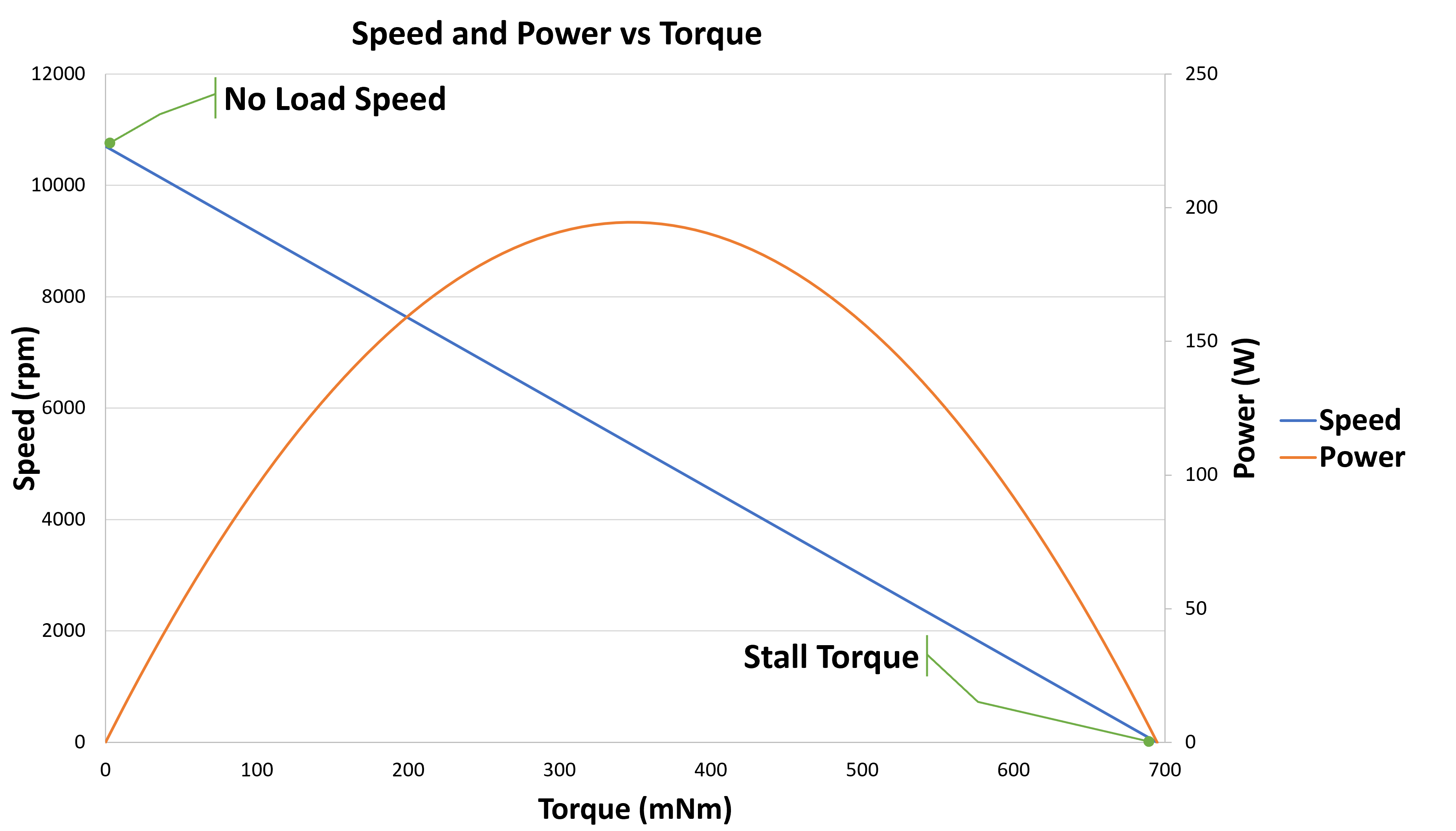
From the data sheet, take the no load speed (row 2) and the stall torque (row 7) for the chosen winding. For the 24 V winding these are 10 700 rpm and 695 mNm, which give the two end points of the speed–torque line.
\[ P_{MECH} = \frac{\pi}{30}\, n\, T_m \]
Use the equation of the line to determine values for \(n\) and \(T_m\).
Current and efficiency against torque
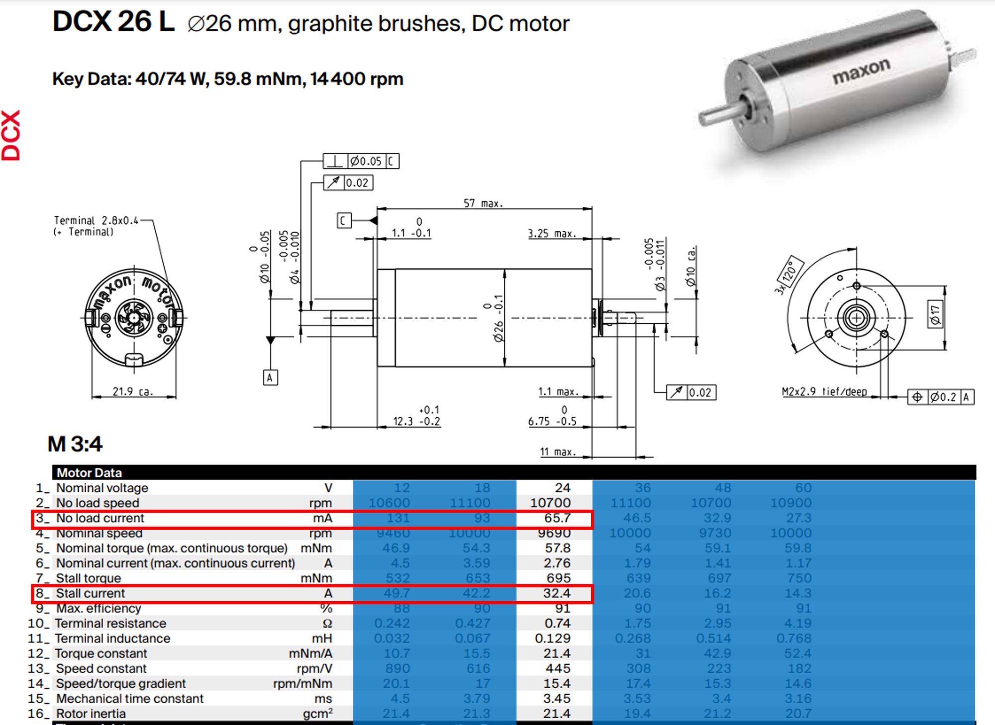
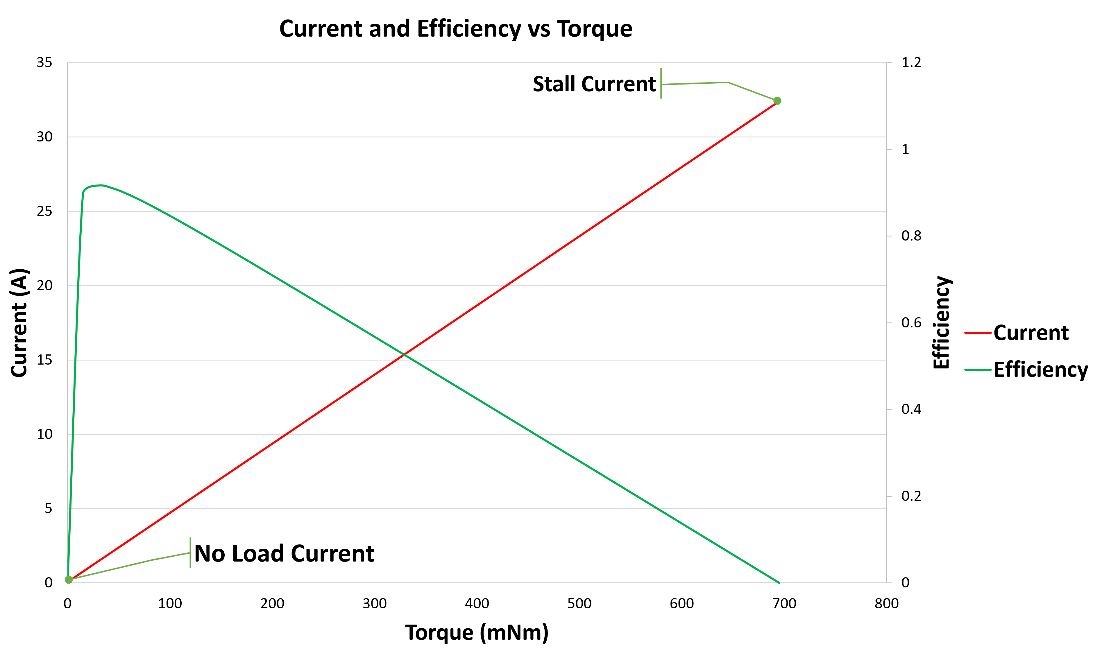
Next take the no load current (row 3) and the stall current (row 8). For the 24 V winding these are 65.7 mA and 32.4 A, which give the two end points of the current–torque line.
\[ \eta = \frac{P_{MECH}}{v_{in}\, i_a} \]
Use the equation of the line to determine \(i_a\) values for a given \(T_m\).
Explore the operating point
Interactive diagram: drag across the charts to set the load torque and see the speed, current, power and efficiency worked out from the data sheet; change the supply voltage or the winding; you can also load another maxon data sheet PDF or type its values in · Open full screen ↗
Knowledge Check
Q1. Which characteristic motor data are strongly winding-dependent, and which are almost independent of the winding?
Answer
Winding-dependent: terminal resistance \(R_a\), terminal inductance \(L\), torque constant \(K_m\), speed constant \(K_b\). Almost independent: speed–torque gradient, mechanical time constant \(\tau_m\), rotor inertia \(J\).
Q2. A motor has a torque constant of 25 mN·m/A. What current does it draw to produce 100 mN·m, ignoring the no-load current?
Answer
\(i_a = T_m/K_m = 100/25 = 4\) A.
Q3. A motor has a speed constant of 400 rpm/V. What is its approximate no-load speed at 12 V?
Answer
\(n_0 = K_s V = 400 \times 12 = 4800\) rpm.
Q4. How does increasing the supply voltage change the speed–torque line?
Answer
The line moves up, parallel to itself: the no-load speed rises in proportion to the voltage, while the gradient \(\Delta n/\Delta T_m\) is unchanged.
Q5. What distinguishes a “strong” motor from a “weak” one on its speed–torque curve?
Answer
A strong motor (strong magnet, larger motor) has a flat speed–torque line (low \(\Delta n/\Delta T_m\)), so its speed is insensitive to load. A weak motor has a steep line and slows down much more under load.
Q6. Compare a low-resistance winding with a high-resistance winding.
Answer
Low resistance: thick wire, few turns, low rated voltage, high currents, high specific speed, low specific torque. High resistance: thin wire, many turns, high rated voltage, low currents, low specific speed, high specific torque.
Q7. A motor runs at 6000 rpm and delivers 50 mN·m. What is its mechanical output power?
Answer
\(P = \dfrac{\pi}{30}\,n\,T_m = \dfrac{\pi}{30} \times 6000 \times 0.05 = 31.4\) W.
Q8. At what torque does a DC motor deliver its maximum mechanical power, and roughly what is its efficiency there?
Answer
At half the stall torque (and half the no-load speed). The efficiency there is just under 50%, because the copper loss equals the mechanical power.
Q9. Why is maximum efficiency reached at a much lighter load than maximum power?
Answer
Copper loss grows with the square of the current (and so of the torque), while useful power rises more slowly and then falls. Efficiency is highest at light load, where the copper loss is small compared with the output; by half the stall torque the losses equal the output.
Q10. A 24 V motor draws 2 A at a speed of 4000 rpm while delivering 90 mN·m. What is its efficiency?
Answer
\(P_{mech} = \dfrac{\pi}{30} \times 4000 \times 0.09 = 37.7\) W; \(P_{in} = 24 \times 2 = 48\) W; \(\eta = 37.7/48 = 78.5\%\).