Lecture 3: DC Motor Start-up
Speed/Voltage from First Principles
Up to now, we have looked at output torque for input current at motor steady state, i.e. the motor has already reached its final angular velocity. This approach is useful during the systems design phase.
Faced with characterising an existing system, an alternative approach is to look at angular velocity over time for a fixed voltage.
This form of analysis involves deriving fundamental equations from first principles and then applying them to experimentally derived data to get information on how the motor system would respond to different input criteria. This can be useful because:
- Any motor is typically connected to a load or drive system (belts, pulleys, fans, pumps etc.). This approach allows the engineer to derive the time response of the entire system as opposed to just the motor.
- The rated power for a given motor is given at nominal currents and torque. It is not atypical that the operating point for a motor/motorised system is not exactly at this point.
- The data for the motor may not be available, leaving experimental determination of the motor constants the most appropriate option.
Analysis of angular velocity \(\omega(t)\) for a given applied voltage \(v_{in}\)
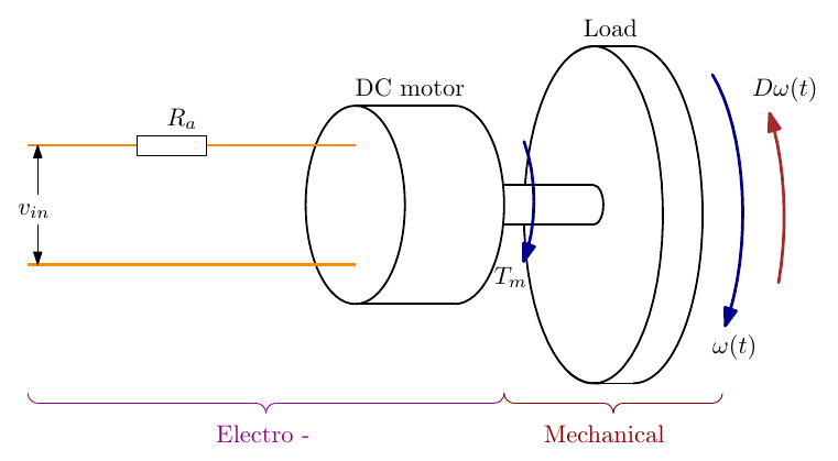
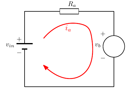
This consists of linking the mechanical and electrical equations together via the expression for torque \(T_m\).
Mechanical System
\[ J\,\frac{d\omega}{dt} = T_m - D\,\omega(t) \]
\[ T_m = J\,\frac{d\omega}{dt} + D\,\omega(t) \]
Where:
- \(J\) = Inertia of the load (\(\text{kg·m}^2\)). > Note: Formulas for mass moment of inertia for different shapes can be found in the Maxon formula book.
- \(T_m\) = Torque applied to the load (\(\text{N·m}\))
- \(D\) = Viscous friction (\(\text{N·m}/\text{rad/s}\))
- \(\omega(t)\) = Angular velocity of the load (\(\text{rad/s}\))
Electrical System
\[ i_a = \frac{v_{in} - \varepsilon_b}{R_a} \]
Where:
- \(i_a\) = Armature current (A)
- \(v_{in}\) = Applied voltage (V)
- \(R_a\) = Armature resistance (\(\Omega\))
- \(\varepsilon_b\) = Back e.m.f (V)
In relation to back e.m.f — remember Lenz’s law. We are moving a conductor in a magnetic field; the current generated in this conductor opposes the movement and is a function of change in the magnetic field, i.e. how fast the conductor is moving.
Torque and back e.m.f. constants
We have also seen how the force generated in a conductor is a function of the applied current (\(\mathbf{F} = BiL\sin\theta\)). In terms of motor torque we can say:
\[ i_a \propto T_m \]
\[ K_m\, i_a = T_m \]
Where \(K_m\) is known as the motor constant (\(\text{N·m}/\text{A}\)).
In relation to back e.m.f. \(\varepsilon_b\), we know that this is proportional to the speed of the conductor through the magnetic field:
\[ \varepsilon_b \propto \omega(t) \]
\[ \varepsilon_b = K_b\, \omega(t) \]
Where \(K_b\) is known as the back e.m.f constant (\(\text{V}/\text{rad/s}\)).
Putting these equations together
\[ i_a = \frac{T_m}{K_m} = \frac{v_{in} - K_b\,\omega(t)}{R_a} \]
\[ T_m = K_m\left(\frac{v_{in} - K_b\,\omega(t)}{R_a}\right) \]
\[ T_m = \frac{K_m\, v_{in} - K_m K_b\,\omega(t)}{R_a} \]
\[ T_m = \frac{K_m}{R_a}\,v_{in} - \frac{K_m K_b}{R_a}\,\omega(t) \]
Electro-Mechanical System
Equating both expressions for torque gives:
\[ J\,\frac{d\omega}{dt} + D\,\omega(t) = \frac{K_m}{R_a}\,v_{in} - \frac{K_m K_b}{R_a}\,\omega(t) \]
\[ J\,\frac{d\omega}{dt} + D\,\omega(t) + \frac{K_m K_b}{R_a}\,\omega(t) = \frac{K_m}{R_a}\,v_{in} \]
\[ J\,\frac{d\omega}{dt} + \left(D + \frac{K_m K_b}{R_a}\right)\omega(t) = \frac{K_m}{R_a}\,v_{in} \]
\[ \frac{d\omega}{dt} + \left(\frac{D}{J} + \frac{K_m K_b}{J R_a}\right)\omega(t) = \frac{K_m}{J R_a}\,v_{in} \]
Letting
\[ \alpha = \frac{D}{J} + \frac{K_m K_b}{J R_a} \qquad \text{and} \qquad K = \frac{K_m}{J R_a} \]
we can say:
\[ \frac{d\omega}{dt} + \alpha\,\omega(t) = K\, v_{in} \]
Step Response
The expression \(\dfrac{d\omega}{dt} + \alpha\,\omega(t) = K\,v_{in}\) is a first order differential equation and can be solved for constant \(v_{in}\) (starting from rest, \(\omega(0) = 0\)) to give:
\[ \omega(t) = \frac{v_{in} K}{\alpha}\left(1 - e^{-\alpha t}\right) \]
Plotting this curve over time gives:
Interactive diagram: change vin, Ra, Km, J and D and run the start-up, at whatever replay speed you like, to see ω(t), the armature current and the back emf; a DCX 26 L preset reproduces the data sheet’s 3.45 ms mechanical time constant; “Find the constants” works back from a measured curve to J and D · Open full screen ↗
- The final (steady-state) angular velocity is \(\omega_{\infty} = \dfrac{v_{in} K}{\alpha}\).
- At \(t = 1/\alpha\) (one time constant) the speed has reached \(1 - e^{-1} \approx 0.63\) of its final value.
Points to Note
- The shape of the graph above is likely relatively intuitive. What this is saying is that if a constant voltage is applied to a motor, the motor speed will increase and will gradually settle at a final angular velocity.
- What this analysis does show is that the length of time it takes to get to the final speed, and what that angular velocity is, is dependent on the applied voltage and a number of motor properties such as wire resistance, inertia of the load being driven etc.
- It is possible to obtain this curve experimentally and determine key motor properties that can then allow the motor suitability for specific applications to be assessed. This approach is particularly useful for closed loop control scenarios where defined speed and/or position of the motor is required.
Knowledge Check
Q1. Write the mechanical equation of the motor and load, and explain each term.
Answer
\(J\,\dfrac{d\omega}{dt} = T_m - D\,\omega(t)\): the inertia \(J\) times the angular acceleration equals the motor torque \(T_m\) minus the viscous friction torque \(D\omega\).
Q2. Why does the armature current fall as the motor speeds up?
Answer
The back e.m.f. \(\varepsilon_b = K_b\omega\) rises with speed, so the voltage left to drive current through the armature resistance, \(v_{in} - K_b\omega\), falls: \(i_a = (v_{in} - K_b\omega)/R_a\).
Q3. Write the expressions for \(\alpha\) and \(K\) in the first-order model, and the solution for \(\omega(t)\).
Answer
\(\alpha = \dfrac{D}{J} + \dfrac{K_mK_b}{J R_a}\), \(K = \dfrac{K_m}{J R_a}\), and \(\omega(t) = \dfrac{v_{in}K}{\alpha}\left(1 - e^{-\alpha t}\right)\).
Q4. What fraction of the final speed has the motor reached after one time constant, \(t = 1/\alpha\)? After five?
Answer
\(1 - e^{-1} \approx 63\%\) after one time constant; \(1 - e^{-5} \approx 99.3\%\) after five.
Q5. If the load inertia \(J\) is doubled (with negligible friction), what happens to the time constant and the final speed?
Answer
With \(D\) negligible, \(\alpha \approx K_mK_b/(JR_a)\), so the time constant doubles. The final speed \(v_{in}K/\alpha \approx v_{in}/K_b\) is unchanged.
Q6. What effect does increasing the viscous friction \(D\) have on the final speed?
Answer
It lowers the final speed (and shortens the time constant), because \(\alpha\) increases while \(K\) is unchanged, so \(\omega_\infty = v_{in}K/\alpha\) falls.
Q7. In SI units, how are \(K_m\) (N·m/A) and \(K_b\) (V/(rad/s)) related?
Answer
They are numerically equal: both express the same electromechanical coupling.
Q8. Give two reasons for characterising a motor from its measured step response.
Answer
Any two of: it gives the response of the whole system (motor plus load and drive), not just the motor; the operating point may differ from the rated point; the motor’s data may not be available, so the constants must be found experimentally.
Q9. A motor and load reach 63% of their final speed of 300 rad/s in 50 ms at \(v_{in} = 12\) V. Find \(\alpha\) and \(K\).
Answer
\(\alpha = 1/0.05 = 20\ \text{s}^{-1}\); \(K = \alpha\,\omega_\infty/v_{in} = 20 \times 300/12 = 500\) rad·s⁻²·V⁻¹.