Performance of Assembly Systems
Chapter 18 · Part V: Performance and Economics · Source: Lecture 17
In automatic assembly machines, downtime or malfunction can cause serious loss of production. This is worse for indexing machines, where the whole line stops when one station malfunctions. In free transfer systems, the other stations can keep working as long as the buffers allow. A major cause of shutdowns is defective parts; this chapter analyses how part quality affects output.
18.1 Indexing machine
Consider an indexing machine with \(n\) workheads and a cycle time of \(t\) seconds. Let:
- \(x\) = ratio of defective parts (assumed the same at every workhead)
- \(m\) = ratio of defective parts that cause machine stoppage
- \(T\) = time to fix the machine after a stoppage
Time to assemble \(N\) parts = \(Nt\). Total downtime for \(N\) assemblies = \(mxNTn\).
\[\text{Proportion of downtime} = \frac{\text{downtime}}{\text{assembly time} + \text{downtime}} = \frac{mxNTn}{Nt + mxNTn} = \frac{mxn}{\dfrac{t}{T} + mxn}\]
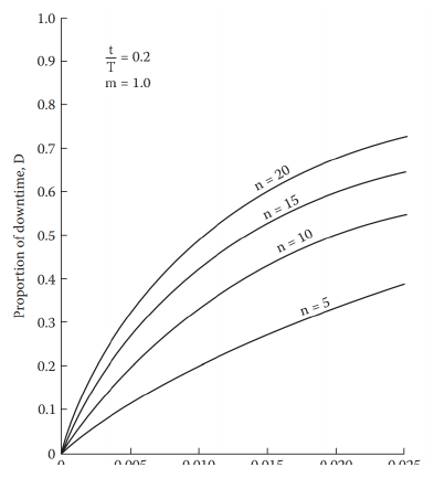
Figure 18.1: Proportion of downtime vs x, for t/T = 0.2 and m = 1 (t = 6 s, T = 30 s).
For a typical defective-part ratio of 0.01, too many workheads becomes uneconomical. When designing an automated system, a downtime of 50% is often assumed to allow for problems on the line.
Production time
- If \(m < 1\), some defective parts pass through and produce faulty assemblies; the time lost on each is effectively one machine cycle.
- \(mxnN\) = number of parts causing stoppage in \(N\) assemblies.
- \((1 - m)xnN\) = number of faulty assemblies produced.
- \(N - (1 - m)xnN\) = number of acceptable assemblies per \(N\) made.
- Average production time = total time ÷ number of acceptable assemblies:
\[t_{pr} = \frac{Nt + mxnNT}{N - (1 - m)xnN} = \frac{t + mxnT}{1 - (1 - m)xn}\]
With \(x = 0.01\), \(t = 6\) s, \(T = 30\) s, \(n = 10\):
\[t_{pr} = \frac{6 + 3m}{0.9 + 0.1m} = \frac{30(2 + m)}{9 + m}\]
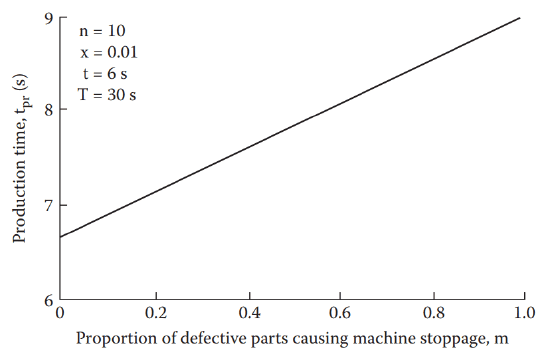
Figure 18.2: Production time rises with m.
To maximise production rate, let defective assemblies pass through rather than stopping the line to remove them. If \(m = 1\) (defects always stop the machine):
\[t_{pr} = t + xnT\]
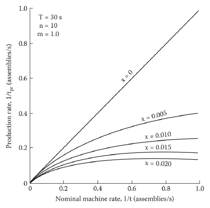
Figure 18.3: Production rate of good assemblies vs nominal machine rate, for T = 30 s, n = 10, m = 1.
For \(x = 0\) there is no downtime, so \(t_{pr} = t\). In practice \(x\) is typically 0.005–0.02, and in this range high machine rates don’t greatly increase the output of good assemblies, because much of the time is spent clearing stoppages caused by faulty parts. There is no point running the machine at its maximum rate, as the machine itself will start causing further problems.
18.2 Free transfer machine
Downtime on a free transfer machine is lower than on an indexing machine when buffers are used. Assume all workheads have cycle time \(t\), part quality \(x\) is the same at all workheads, and the buffers between workheads hold up to \(b\) assemblies, with average contents \(a_1 \dots a_4\).
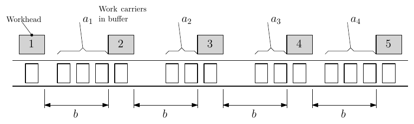
Figure 18.4: Five workheads separated by buffers of capacity b with average contents \(a_1\)–\(a_4\).
Causes of stoppage at workhead 2
- A defective part at station 2 stops it for \(T\) seconds until cleared.
- A blockage at station 1 long enough to empty the buffer between stations 1 and 2. Station 2 can keep going for \(a_1t\), so its downtime is \(T - a_1t\).
- A blockage at station 3 long enough to fill the buffer between stations 2 and 3. Station 2 can keep going for \((b - a_2)t\), so its downtime is \(T - (b - a_2)t\).
For cause 3, the downtime over \(N\) assemblies is \(Nx[T - (b - a_2)t]\).
Knock-on effects. If station 4 goes down, station 3 is down for \(Nx[T - (b - a_3)t] = NxT'\), so station 2 has downtime
\[Nx[T' - (b - a_2)t] = Nx[T - (2b - a_2 - a_3)t]\]
Summing the stoppages from all workheads at workhead 2:
\[d_2 = Nx[(T - a_1t) + T + (T - (b - a_2)t) + (T - (2b - a_2 - a_3)t) + (T - (3b - a_2 - a_3 - a_4)t)]\]
Downtime table
\(d_i/Nx\) at workhead \(i\) (rows), due to a stoppage at each workhead (columns):
| At ↓ / due to → | 1st | 2nd | 3rd | 4th | 5th |
|---|---|---|---|---|---|
| 1st | \(T\) | \(T - (b - a_1)t\) | \(T - (2b - a_1 - a_2)t\) | \(T - (3b - a_1 - a_2 - a_3)t\) | \(T - (4b - a_1 - a_2 - a_3 - a_4)t\) |
| 2nd | \(T - a_1t\) | \(T\) | \(T - (b - a_2)t\) | \(T - (2b - a_2 - a_3)t\) | \(T - (3b - a_2 - a_3 - a_4)t\) |
| 3rd | \(T - (a_1 + a_2)t\) | \(T - a_2t\) | \(T\) | \(T - (b - a_3)t\) | \(T - (2b - a_3 - a_4)t\) |
| 4th | \(T - (a_1 + a_2 + a_3)t\) | \(T - (a_2 + a_3)t\) | \(T - a_3t\) | \(T\) | \(T - (b - a_4)t\) |
| 5th | \(T - (a_1 + a_2 + a_3 + a_4)t\) | \(T - (a_2 + a_3 + a_4)t\) | \(T - (a_3 + a_4)t\) | \(T - a_4t\) | \(T\) |
Note: any term that comes out negative is omitted. E.g. if \((b - a_1)t > T\), no downtime is incurred at station 1 from a blockage at station 2.
Effect of buffer size b on average buffer contents
(\(t = 6\) s, \(T = 30\) s)
| \(b\) | Omit in \(d_1\) | \(d_2\) | \(d_3\) | \(d_4\) | \(d_5\) | \(a_1/b\) | \(a_2/b\) | \(a_3/b\) | \(a_4/b\) |
|---|---|---|---|---|---|---|---|---|---|
| 0, 1, 2 | – | – | – | – | – | 4/5 | 3/5 | 2/5 | 1/5 |
| 3 | 5 | 5 | – | 1 | 1 | 3/4 | 7/12 | 5/12 | 1/4 |
| 4 | 4, 5 | 5 | 1, 5 | 1 | 1, 2 | 3/4 | 1/2 | 1/2 | 1/4 |
| 5, 6 | 4, 5 | 4, 5 | 1, 5 | 1, 2 | 1, 2 | 2/3 | 5/9 | 4/9 | 1/3 |
| 7 | 3, 4, 5 | 4, 5 | 1, 5 | 1, 2 | 1, 2 | 22/35 | 19/35 | 16/35 | 13/35 |
| 8 | 3, 4, 5 | 4, 5 | 1, 5 | 1, 2 | 1, 2, 3 | 23/40 | 21/40 | 19/40 | 17/40 |
| 9 | 3, 4, 5 | 4, 5 | 1, 5 | 1, 2 | 1, 2, 3 | 24/45 | 23/45 | 22/45 | 21/45 |
| 10 | 2, 3, 4, 5 | 1, 3, 4, 5 | 1, 2, 4, 5 | 1, 2, 3, 5 | 1, 2, 3, 4 | 1/2 | 1/2 | 1/2 | 1/2 |
Equalising downtime
Find the buffer contents that give the same average downtime at every workhead, which maximises overall throughput. Setting \(d_1 = d_2 = d_3 = d_4 = d_5 = d\):
\[\begin{aligned} d &= 5T - 10bt + 4a_1t + 3a_2t + 2a_3t + a_4t \\ d &= 5T - 6bt - a_1t + 3a_2t + 2a_3t + a_4t \\ d &= 5T - 3bt - a_1t - 2a_2t + 2a_3t + a_4t \\ d &= 5T - bt - a_1t - a_2t - 3a_3t + a_4t \\ d &= 5T - a_1t - 2a_2t - 3a_3t - 4a_4t \end{aligned}\]
Equation 1 − equation 2: \(-4bt + 5a_1t = 0 \Rightarrow a_1 = \dfrac{4b}{5}\). Similarly \(a_2 = \dfrac{3b}{5}\), \(a_3 = \dfrac{2b}{5}\), \(a_4 = \dfrac{b}{5}\).
For \(T/t = 5\), all the equations are valid for \(b \le 2\), giving
\[\frac{d}{Nx} = (25 - 4b)t \qquad \text{Proportion of downtime} = \frac{(25 - 4b)x}{1 + (25 - 4b)x}\]
For \(b \ge 10\) with \(T/t = 5\), every cross-term is omitted, and the downtime at a station comes only from malfunctions at that station:
\[\frac{d}{Nx} = T \qquad \text{Proportion of downtime} = \frac{NxT}{Nt + NxT} = \frac{5x}{1 + 5x}\]
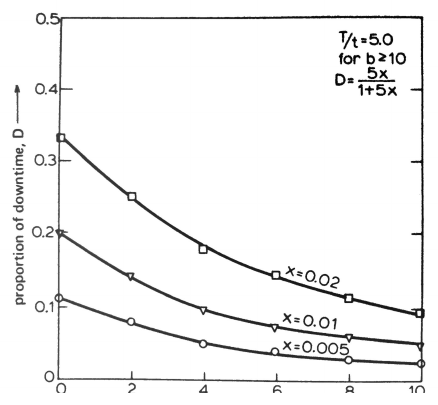
Figure 18.5: Proportion of downtime vs buffer size for x = 0.005, 0.01 and 0.02.
In theory, when \(b \ge 2T/t\) the workheads are isolated from each other and machine downtime approaches workhead downtime. Practical constraints usually lead to a buffer size of \(b = T/t\).
Note: \(d = NxT\) and \(\Sigma d = nNxT\), which looks like an indexing machine with \(m = 1\). But downtime can happen in parallel, so the individual \(d\) values aren’t simply added: downtimes at different stations may overlap.
Key points
- Indexing machine: downtime proportion \(= mxn/(t/T + mxn)\); letting defects pass (\(m < 1\)) maximises the production rate.
- With realistic \(x\) (0.005–0.02), raising the machine rate gives diminishing returns.
- Free transfer: buffers decouple stations; equal downtime needs \(a_i = (5-i)b/5\), and \(b \approx T/t\) is a practical buffer size.
Interactive applets
Each applet runs in the page; use Open full screen for more room, or open all of this chapter’s applets together.
Applet 18.1 · Indexing machine downtime calculator
Sliders for \(n\), \(x\), \(m\), \(t\) and \(T\); live plots of downtime proportion vs \(x\) (one curve per \(n\)) and \(t_{pr}\) vs \(m\), with the operating point marked.
Teaches: Figures 18.1–18.3 interactively. · Open full screen ↗
Applet 18.2 · “Should I stop for defects?” explorer
Compare good-assembly output for \(m = 0\), \(0.5\) and \(1\) at the same settings, including the cost of faulty assemblies (an optional slider for rework cost).
Teaches: Why letting defects through can maximise throughput, and when it doesn’t. · Open full screen ↗
Applet 18.3 · Free transfer line discrete-event simulator
A five-station animated line with random defect stoppages (\(x\), \(T\)) and adjustable buffer size \(b\); buffers fill and empty visually and blocked or starved stations turn red. Compares simulated downtime with the analytical table.
Teaches: Starvation and blocking, knock-on effects, and the \(b = T/t\) rule. · Open full screen ↗
Applet 18.4 · Buffer sizing optimiser
Add a cost per buffer slot and a value per assembly; the applet finds the \(b\) that maximises profit.
Teaches: Engineering trade-offs beyond pure throughput. · Open full screen ↗