Karnaugh Maps and Problem Breakdown
Chapter 3 · Part I: Logic Control Fundamentals · Sources: Lectures 2 and 3
3.1 The idea behind Karnaugh maps
A Karnaugh map (K-map) is a graphical method of simplifying logic expressions. It relies on two laws:
- Inclusion theorem: \(A + \overline{A} = 1\)
- Characteristic theorem: \(X.1 = X\)
K-maps group terms that differ only in one complemented variable, e.g.
\[A.B.C + A.B.\overline{C} = A.B.(C + \overline{C}) = A.B.1 = A.B\]
3.2 Two-variable maps
To minimise \(A.\overline{B} + A.B\):
- Draw a grid representing all possible variable states.
- Enter the expression’s states: \(A.\overline{B} \to 10\), \(A.B \to 11\).
- Group adjacent 1s, and read off the variables that don’t change within the group.
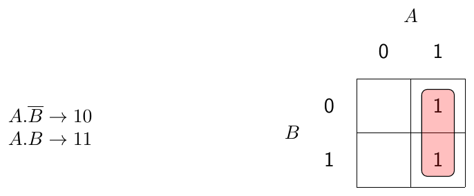
Figure 3.1: \(A.\overline{B} + A.B = A\).
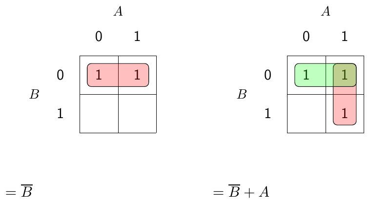
Figure 3.2: Further examples: \(=\overline{B}\) and \(=\overline{B} + A\).
Any group of \(2^n\) adjacent cells can be combined, where \(n\) is a positive integer: two, four, eight cells and so on.
3.3 Three- and four-variable maps
The axes use Gray-code ordering (00, 01, 11, 10), so adjacent cells differ by exactly one variable.
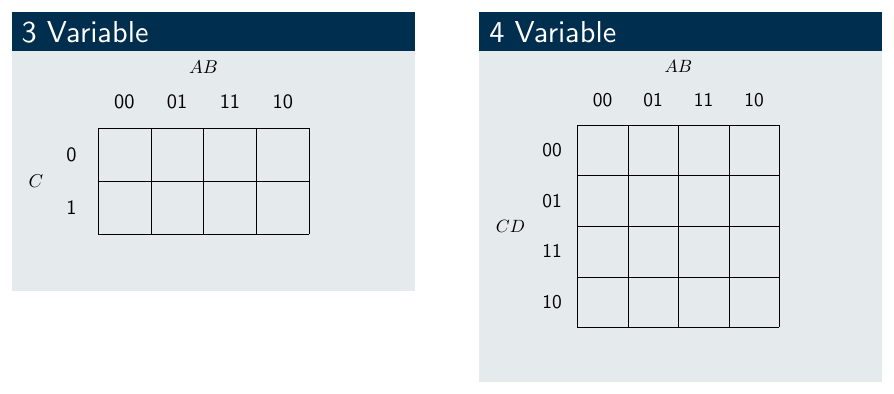
Figure 3.3: Three-variable and four-variable K-map layouts.
Worked exercise
Simplify the 13-term expression:
\[Y = \overline{A}.\overline{B}.\overline{C}.D + \overline{A}.\overline{B}.C.D + \overline{A}.B.\overline{C}.\overline{D} + \overline{A}.B.\overline{C}.D + \overline{A}.B.C.D + A.B.\overline{C}.\overline{D} + A.B.\overline{C}.D + A.B.C.D + A.B.C.\overline{D} + A.\overline{B}.\overline{C}.\overline{D} + A.\overline{B}.\overline{C}.D + A.\overline{B}.C.D + A.\overline{B}.C.\overline{D}\]
| AB → / CD ↓ | 00 | 01 | 11 | 10 |
|---|---|---|---|---|
| 00 | 1 | 1 | 1 | |
| 01 | 1 | 1 | 1 | 1 |
| 11 | 1 | 1 | 1 | 1 |
| 10 | 1 | 1 |
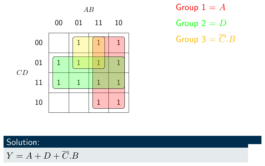
Figure 3.4: Grouping the exercise.
- Group 1 = \(A\) (columns 11 and 10)
- Group 2 = \(D\) (rows 01 and 11)
- Group 3 = \(\overline{C}.B\) (columns 01 and 11, rows 00 and 01)
Solution: \(Y = A + D + \overline{C}.B\)
3.4 Points to note
Edges wrap around. The map is a 2-D graph, but the left and right edges meet, and so do the top and bottom.
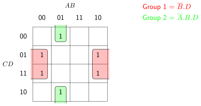
Figure 3.5: Group 1 = \(\overline{B}.D\) (left and right edges meet); Group 2 = \(\overline{A}.B.\overline{D}\) (top and bottom edges meet).
Correction: the slide labels Group 2 as \(\overline{A}.B.D\), but these cells lie in rows CD = 00 and 10, where D = 0, so the bar over D is needed.
The four corners touch. The four corner cells form one group, \(\overline{B}.\overline{D}\).
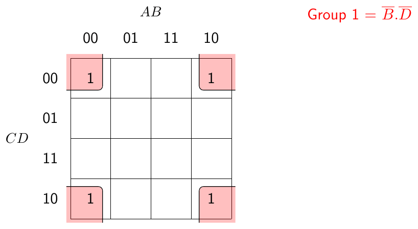
Figure 3.6: Corner grouping.
“Don’t care” states. Some input conditions are irrelevant or physically impossible. They are marked X and can be treated as 1 or 0, whichever gives the simpler expression. (Note that the axes here are AC across and BD down.)
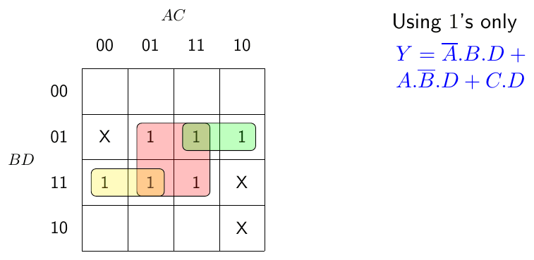
Figure 3.7: Using 1s only, \(Y = \overline{A}.B.D + A.\overline{B}.D + C.D\).
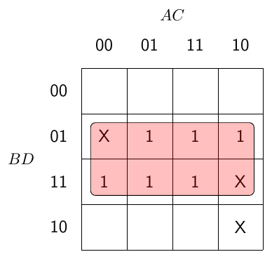
Figure 3.8: Using 1s and X terms, \(Y = D\).
3.5 Example: automatic work station
- An automatic work station cycles (Y = 1) when the power P is on and the “cycle ready” indicator C is on.
- The machine is switched on with a spring-return Go switch G and off with a spring-return Stop switch S.
- The Stop switch takes precedence over the Go switch.
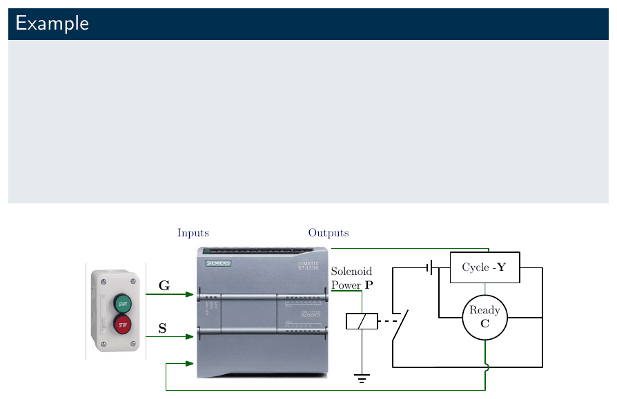
Figure 3.9: Work station with Go/Stop buttons, PLC, power solenoid and cycle-ready indicator.
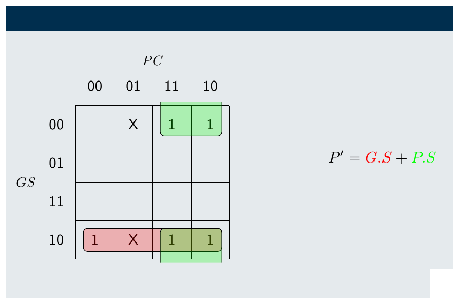
Inputs: G (Go pressed), S (Stop pressed), P (power on), C (cycle ready on). Outputs: \(P'\) (power on), Y (station cycles).
| G | S | P | C | P′ | Y | Comment |
|---|---|---|---|---|---|---|
| 0 | 0 | 0 | 0 | 0 | 0 | |
| 0 | 0 | 0 | 1 | X | X | State can’t exist |
| 0 | 0 | 1 | 0 | 1 | 0 | |
| 0 | 0 | 1 | 1 | 1 | 1 | |
| 0 | 1 | 0 | 0 | 0 | 0 | |
| 0 | 1 | 0 | 1 | 0 | 0 | Would be X, but S is on |
| 0 | 1 | 1 | 0 | 0 | 0 | |
| 0 | 1 | 1 | 1 | 0 | 0 | |
| 1 | 0 | 0 | 0 | 1 | 0 | |
| 1 | 0 | 0 | 1 | X | X | State can’t exist |
| 1 | 0 | 1 | 0 | 1 | 0 | |
| 1 | 0 | 1 | 1 | 1 | 1 | |
| 1 | 1 | 0 | 0 | 0 | 0 | |
| 1 | 1 | 0 | 1 | 0 | 0 | Would be X, but S is on |
| 1 | 1 | 1 | 0 | 0 | 0 | |
| 1 | 1 | 1 | 1 | 0 | 0 |
| K-map for \(P'\) | K-map for \(Y\) |
|---|---|
 |
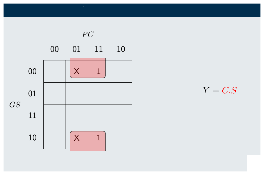 |
\[P' = G.\overline{S} + P.\overline{S} \qquad Y = C.\overline{S}\]
3.6 Problem breakdown
- A 2-D K-map can only handle 4 variables.
- 3-D K-maps exist and can be drawn in 2-D, but they are cumbersome.
- If possible, break the system into subsystems to simplify the analysis.
Example: pneumatic press
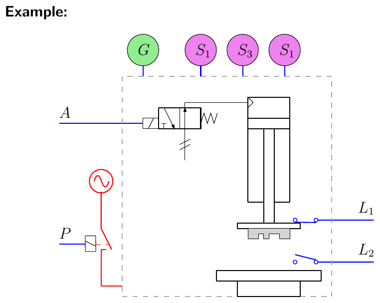
Figure 3.10: Press control problem.
- The power (P) to a press is turned on by a start button G and turned off by any one of three stop buttons S1, S2 or S3.
- The press actuates (A = 1) when limit switch L1 is switched on.
- The press is deactivated when limit switch L2 is switched on, and returns under spring action.
The whole system has 8 inputs (G, S1, S2, S3, L1, L2, P, A), so its truth table would have \(2^8 = 256\) rows! It is easier to break it into subsections.
Stop function. If any of S1–S3 is pressed the power is off, so define a general stop:
\[S = S_1 + S_2 + S_3\]
Power \(P'\): (same structure as the latch in Chapter 2)
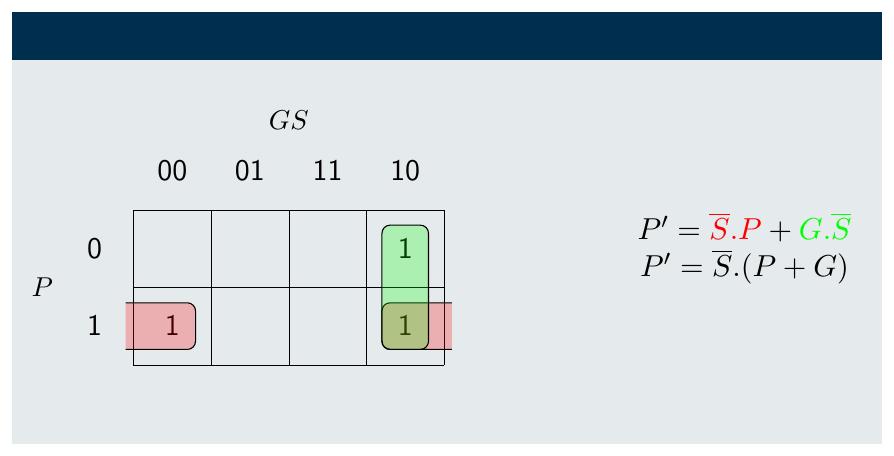
Figure 3.11: \(P' = \overline{S}.P + G.\overline{S} = \overline{S}.(P + G)\).
Press actuation \(A'\), using “don’t care” states:
| P′ | L1 | L2 | A | A′ | Comment |
|---|---|---|---|---|---|
| 0 | x | x | x | X | Power off, so no air supply |
| 1 | 0 | 0 | 0 | 0 | |
| 1 | 0 | 0 | 1 | 1 | |
| 1 | 0 | 1 | 0 | 0 | |
| 1 | 0 | 1 | 1 | 0 | |
| 1 | 1 | 0 | 0 | 1 | |
| 1 | 1 | 0 | 1 | 1 | |
| 1 | 1 | 1 | x | X | L1 and L2 can’t both be on |
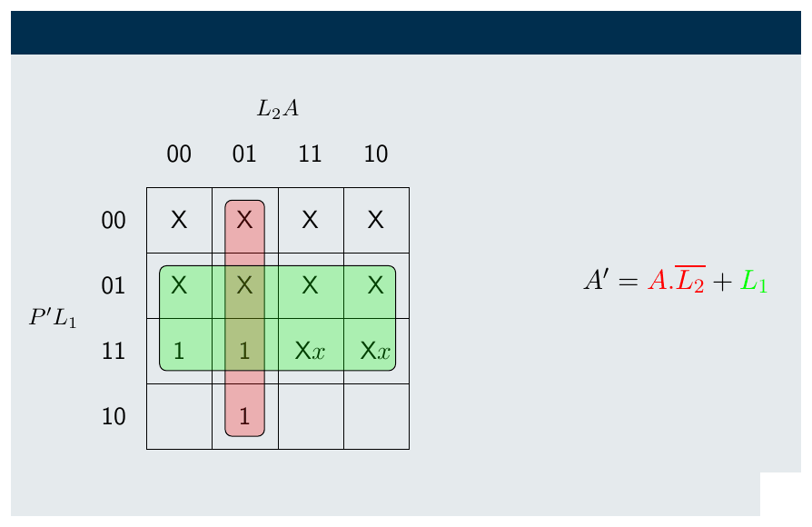
Figure 3.12: \(A' = A.\overline{L_2} + L_1\).
Potential issues with “don’t care”
Always consider whether a “don’t care” assumption is practical, and how to fail safe:
- The X states could be regarded as impossible, but for safety they could be set to 0, since \(P' = 0\) means a stop button has been pressed. From a safety point of view, a Stop press should force all outputs to 0 rather than leaving them “don’t care”.
- L1 = L2 = 1 should never happen; it would only occur through a fault, so do not actuate.
- One or more switches stuck: perhaps raise an alarm.
Fail-safe truth table: every row with \(P' = 0\), and both rows with L1 = L2 = 1, give \(A' = 0\).
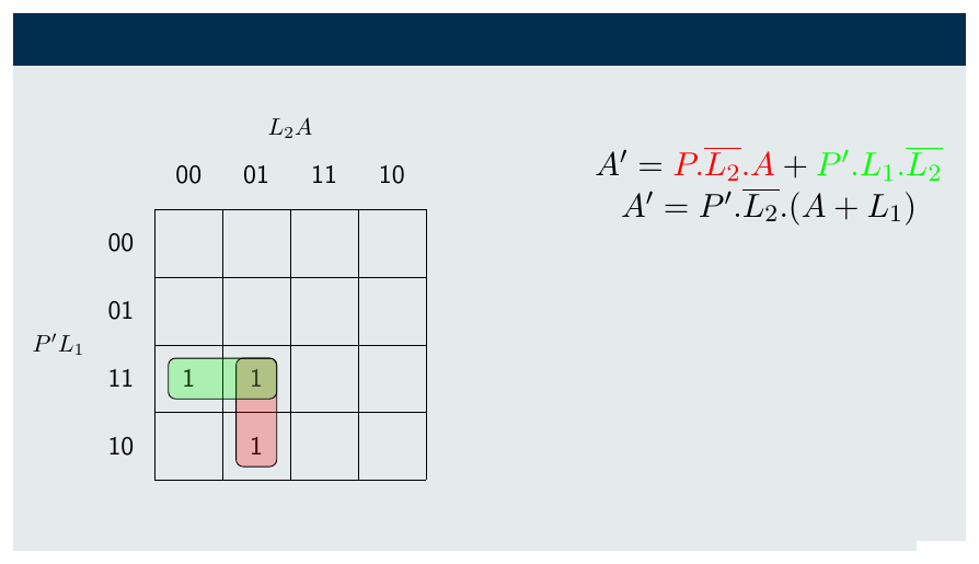
Figure 3.13: Fail-safe solution.
\[A' = P'.\overline{L_2}.A + P'.L_1.\overline{L_2} = P'.\overline{L_2}.(A + L_1)\]
Substituting \(P' = \overline{S}.(P + G)\) and \(S = S_1 + S_2 + S_3\):
\[A' = \overline{S_1 + S_2 + S_3}\,.(P + G).\overline{L_2}.(A + L_1)\]
Key points
- Group 1s (and helpful Xs) in rectangles of \(2^n\) cells, as large as possible; edges and corners wrap.
- Use “don’t care” for impossible states, but check fail-safe behaviour before relying on it.
- Break large problems into subsystems and substitute the results back in.
Interactive applets
Each applet runs in the page; use Open full screen for more room, or open all of this chapter’s applets together.
Applet 3.1 · K-map solver and trainer
Click cells of a 2-, 3- or 4-variable map to cycle 0 → 1 → X, then draw group rectangles. The applet checks each group is a valid \(2^n\) block (including wrap-around), shows the term it produces, and compares the learner’s answer with the optimal one.
Teaches: Grouping rules, wrap-around, corners and don’t-cares. · Open full screen ↗
Applet 3.2 · Truth table ↔︎ K-map ↔︎ expression linker
Edit any of the three views; the other two update live, and hovering a K-map cell highlights the matching truth-table row.
Teaches: That K-maps are just rearranged truth tables (Gray-code ordering). · Open full screen ↗
Applet 3.3 · Don’t-care vs fail-safe comparator (press example)
Toggle each X state between “don’t care” and “force 0”, then simulate faults (stuck L1, both limit switches on) on an animated press.
Teaches: The safety trade-off of don’t-care states. · Open full screen ↗
Applet 3.4 · Problem decomposition puzzle
Starting from the 256-row press problem, drag inputs into sub-blocks (Stop, Power, Actuation) and see the truth-table size fall.
Teaches: Why and how to break problems down. · Open full screen ↗